Using TubeInflation
[1]:
import pymecht as pmt
import numpy as np
from matplotlib import pyplot as plt
Inflation-extension experiments can be simulated using the TubeInflation class in SampleExperiment module as demonstrated in this example.
Displacement controlled
First, we use the TubeInflation in a simple disp_controlled manner. We start by creating a material and using it to create an experiment sample. Since GOH is an anisotropic material, fiber directions need to be specified before simulation (otherwise an error is raised). In TubeInflation cylinderical coordinates are used in the order of radius, angle, and longitudinal length. For the model to be valid, the fiber directions need to be axially symmetric, which means they should not have
a radial component, and should be symmetric about the circumferential axis. This can be automatically satisfied by using the helper function, which sets the same fiber directions to all material model components, as below.
[2]:
mat_model = pmt.MatModel('Yeoh','goh')
sample = pmt.TubeInflation(mat_model)
pmt.specify_two_fibers(sample,10)
params = sample.parameters
print(sample,params)
Fiber directions set to  10  degrees ( 0.17453292519943295  radians)
An object of type TubeInflationwith radius as input, pressure as output, and the following material
Material model with 2 components:
Component1: YEOH with fiber direction(s):[array([0.        , 0.98480775, 0.17364818]), array([ 0.        ,  0.98480775, -0.17364818])]
Component2: GOH with fiber direction(s):[array([0.        , 0.98480775, 0.17364818]), array([ 0.        ,  0.98480775, -0.17364818])]
 ------------------------------------------------------------------
Keys              Value       Fixed?      Lower bound Upper bound
------------------------------------------------------------------
Ri                1.00        No          0.50        1.50
thick             0.10        No          0.00        1.00
omega             0.00        No          0.00        0.00
L0                1.00        No          1.00        1.00
lambdaZ           1.00        No          1.00        1.00
c1_0              1.00        No          1.00e-04    1.00e+02
c2_0              1.00        No          0.00        1.00e+02
c3_0              1.00        No          0.00        1.00e+02
c4_0              0.00        No          0.00        1.00e+02
k1_1              10.00       No          0.10        30.00
k2_1              10.00       No          0.10        30.00
k3_1              0.10        No          0.00        0.33
------------------------------------------------------------------
By default, the displacement measure (input) is radius and the force measure (output) is pressure. Moreover, we can see that the sample parameters include geometric ones (radius, thickness, length, opening angle omega, and longitudinal stretch lambdaZ) in addition to the material parameters. Next we set the parameter values.
[3]:
params.set('Ri', 9)
params.set('thick', 2)
params.set('omega', 0)
params.set('L0', 1)
params.set('lambdaZ', 1)
params.set('c1_0', 28)
params.set('c2_0', 21)
params.set('c3_0', 8)
params.set('c4_0', 1)
params.set('k1_1',5.)
params.set('k2_1',15)
params.set('k3_1',0.1)
print(params)
------------------------------------------------------------------
Keys              Value       Fixed?      Lower bound Upper bound
------------------------------------------------------------------
Ri                9.00        No          0.50        1.50
thick             2.00        No          0.00        1.00
omega             0.00        No          0.00        0.00
L0                1.00        No          1.00        1.00
lambdaZ           1.00        No          1.00        1.00
c1_0              28.00       No          1.00e-04    1.00e+02
c2_0              21.00       No          0.00        1.00e+02
c3_0              8.00        No          0.00        1.00e+02
c4_0              1.00        No          0.00        1.00e+02
k1_1              5.00        No          0.10        30.00
k2_1              15.00       No          0.10        30.00
k3_1              0.10        No          0.00        0.33
------------------------------------------------------------------
and fix certain parameters (for the parameter fitting etc.).
[4]:
params.fix('Ri')
params.fix('thick')
params.fix('omega')
params.fix('L0')
params.fix('lambdaZ')
print(params)
------------------------------------------------------------------
Keys              Value       Fixed?      Lower bound Upper bound
------------------------------------------------------------------
Ri                9.00        Yes         -           -
thick             2.00        Yes         -           -
omega             0.00        Yes         -           -
L0                1.00        Yes         -           -
lambdaZ           1.00        Yes         -           -
c1_0              28.00       No          1.00e-04    1.00e+02
c2_0              21.00       No          0.00        1.00e+02
c3_0              8.00        No          0.00        1.00e+02
c4_0              1.00        No          0.00        1.00e+02
k1_1              5.00        No          0.10        30.00
k2_1              15.00       No          0.10        30.00
k3_1              0.10        No          0.00        0.33
------------------------------------------------------------------
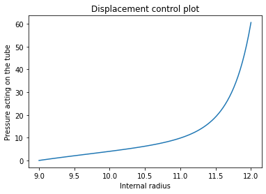
Then we perform the simulation by specifying the deformed internal radius in the disp_controlled method.
[5]:
from matplotlib import pyplot as plt
def_radius = np.linspace(9,12,100)
plt.plot(def_radius,sample.disp_controlled(def_radius,params))
plt.ylabel('Pressure acting on the tube')
plt.xlabel('Internal radius')
plt.title('Displacement control plot')
plt.show()
Force controlled
Inversely, one can specify the force acting on the tube and calculate the deformed internal radius using force_controlled method.
[6]:
from matplotlib import pyplot as plt
force = np.linspace(0,2000,100)
plt.plot(force,sample.force_controlled(force,params))
plt.ylabel('Deformed internal radius')
plt.xlabel('Applied pressure')
plt.title('Force control plot')
plt.show()
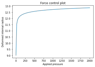
Note that force_controlled uses iterative solver, evaluating the disp_controlled simulation multiple times to find the “displacement” that would result in the applied force (numerically close-enough). Thus, force_controlled is commonly slower than disp_controlled.
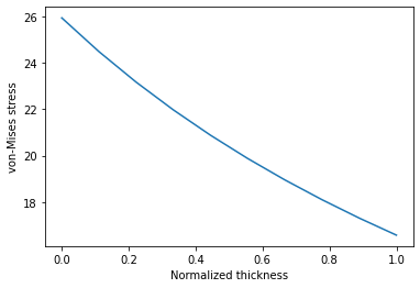
Stress across the thickness
Since the induced stress in a cylinder is non-uniform, we can calculate it using the cauchy_stress method. It takes the disp_measure (by default the deformed inner radius) of the tube and the parameters. The output is a tuple of the normalised thickness xi which has by default 10 points, and stress tensors stress which is a list of the stress tensors at these locations across the thickness.
[7]:
xi,stress = sample.cauchy_stress([10], params)
print(type(xi), type(stress))
print(len(xi), len(stress))
print(stress[0].shape)
<class 'numpy.ndarray'> <class 'list'>
10 10
(3, 3)
For visualisation, we plot the von-Mises stress at each point across the thickness.
[8]:
def von_mises(sigma_list):
    return [sqrt(3./2.)*np.linalg.norm(sigma-np.trace(sigma)/3.*np.eye(3)) for sigma in sigma_list]

plt.plot(xi,von_mises(stress))
plt.xlabel('Normalized thickness')
plt.ylabel('von-Mises stress')
plt.show()
Different force_measures
There are two options for the force_measure argument, as we can see from the helper function.
[9]:
pmt.TubeInflation?
Init signature:
pmt.TubeInflation(
    mat_model,
    disp_measure='radius',
    force_measure='pressure',
)
Docstring:
For simulating uniform axisymmetric inflation of a tube

+-----------+-----------------------------+
| Parameter | Description (default)       |
+===========+=============================+
| Ri        | Internal radius (1)         |
+-----------+-----------------------------+
| thick     | Thickness (0.1)             |
+-----------+-----------------------------+
| omega     | Opening angle (radians) (0) |
+-----------+-----------------------------+
| L0        | Length of sample (1)        |
+-----------+-----------------------------+
| lambdaZ   | Longitudinal stretch (1)    |
+-----------+-----------------------------+

Parameters
----------
mat_model: MatModel
    A material model object of type MatModel
disp_measure: str
    The measure of displacement with the following options:

    * 'stretch' : Ratio of deformed to reference internal radius
    * 'deltar' : Change in internal radius
    * 'radius' : Deformed internal radius (default)
    * 'area' : Deformed internal area

force_measure: str
    The measure of force with the following options:

    * 'force' : Total force acting on the tube length
    * 'pressure' : Internal pressure acting on the tube (default)

File:           /usr/local/lib/python3.9/site-packages/pymecht/SampleExperiment.py
Type:           type
Subclasses:
[10]:
#output pressure (by default)
sample = pmt.TubeInflation(mat_model,force_measure='pressure')
params.set('L0',1)
print(sample.disp_controlled(10,params)) #prints presssure at a deformed radius of 10

params.set('L0',2)
print(sample.disp_controlled(10,params)) #the pressure remains unchanged
4.008308115330826
4.008308115330826
[11]:
#output force, which depends on the length of the tube
sample = pmt.TubeInflation(mat_model,force_measure='force')
params.set('L0',1)
print(sample.disp_controlled(10,params)) #prints force at a deformed radius of 10, which depends on the reference radius and length of the sample

params.set('L0',2)
print(sample.disp_controlled(10,params)) #see the new force, which should be twice
251.84942656895345
503.6988531379069
Different disp_measures
There are four options for the disp_measure argument, as we can see from the helper function above. Thus, one can use different ones when creating the sample. This will result in different outputs from force_controlled. Similarly, the inputs to the disp_controlled will be treated as the chosen disp_measure.
When using force_controlled simulation, an iterative solution is involved, for which an initial guess is required. There is a default value, which may not be reasonable for different disp_measures. Thus, we can explicitly specify the initial guess using x0 argument.
[12]:
sample2 = pmt.TubeInflation(mat_model, disp_measure='stretch', force_measure='pressure')
print('stretch', sample2.force_controlled(10,params,x0=1))

sample2 = pmt.TubeInflation(mat_model, disp_measure='deltar', force_measure='pressure')
print('deltar', sample2.force_controlled(10,params,x0=0))

sample2 = pmt.TubeInflation(mat_model, disp_measure='radius', force_measure='pressure')
print('radius', sample2.force_controlled(10,params,x0=params['Ri'].value))

sample2 = pmt.TubeInflation(mat_model, disp_measure='area', force_measure='pressure')
area = np.pi*(params['Ri'].value)**2 #calculates the lumen area
print('area', sample2.force_controlled(10,params,x0=area))
stretch 1.2239472787140655
deltar 2.0155255084265886
radius 11.015525508426588
area 381.2065144490343
Fiber direction warning
One can manually specify the fiber direction in the material models before using them to create a TubeInflation sample, as follows.
[13]:
mat = pmt.MatModel('yeoh','goh')
mat_models = mat.models
mat_models[1].fiber_dirs = np.array([0,1,1])
sample = pmt.TubeInflation(mat)
print(sample)
An object of type TubeInflationwith radius as input, pressure as output, and the following material
Material model with 2 components:
Component1: YEOH
Component2: GOH with fiber direction(s):[array([0.        , 0.70710678, 0.70710678])]
/usr/local/lib/python3.9/site-packages/pymecht/SampleExperiment.py:536: UserWarning: The TubeInflation assumes that fibers are symmetric w.r.t. axes. This is not satisfied and the results may be spurious.
  warnings.warn("The TubeInflation assumes that fibers are symmetric w.r.t. axes. This is not satisfied and the results may be spurious.")
However, it raises a warning that the fiber directions are not symmetric with respect to the coordinate system, which means there are shear stresses that are being ignored during the simulation. Therefore, to avoid such issues, helper functions specifiy_single_fiber and specify_two_fibers are provided.
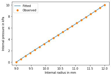
Least square fitting
One can also use TubeInflation instance to perform parameter fitting as demonstrated below. More details on this are provided in the “Using ParamFitter” example.
[14]:
applied_radius = np.linspace(9,12,20)
measured_pressure = np.linspace(0,10,20)

sample = pmt.TubeInflation(mat_model, force_measure='pressure')
pmt.specify_two_fibers(sample,10)

def sim_func(param):
    return sample.disp_controlled(applied_radius,param)

param_fitter = pmt.ParamFitter(sim_func,measured_pressure,params)
Fiber directions set to  10  degrees ( 0.17453292519943295  radians)
Parameter fitting instance created with the following settings
------------------------------------------------------------------
Keys              Value       Fixed?      Lower bound Upper bound
------------------------------------------------------------------
Ri                9.00        Yes         -           -
thick             2.00        Yes         -           -
omega             0.00        Yes         -           -
L0                2.00        Yes         -           -
lambdaZ           1.00        Yes         -           -
c1_0              28.00       No          1.00e-04    1.00e+02
c2_0              21.00       No          0.00        1.00e+02
c3_0              8.00        No          0.00        1.00e+02
c4_0              1.00        No          0.00        1.00e+02
k1_1              5.00        No          0.10        30.00
k2_1              15.00       No          0.10        30.00
k3_1              0.10        No          0.00        0.33
------------------------------------------------------------------

7 parameters will be fitted.
[15]:
res = param_fitter.fit()
   Iteration     Total nfev        Cost      Cost reduction    Step norm     Optimality
       0              1         2.0177e+03                                    2.95e+04
       1              2         3.1888e+02      1.70e+03       4.40e+00       4.18e+03
       2              3         4.5504e+01      2.73e+02       2.56e+00       5.99e+02
       3              4         6.7995e+00      3.87e+01       1.64e+00       9.19e+01
       4              5         1.2549e+00      5.54e+00       2.33e+00       1.72e+01
       5              6         3.0985e-01      9.45e-01       1.61e+00       5.45e+00
       6              7         1.5975e-01      1.50e-01       1.88e+00       2.60e+00
       7              8         1.1851e-01      4.12e-02       3.71e+00       2.81e+00
       8              9         9.1492e-02      2.70e-02       2.38e+00       1.29e+00
       9             10         7.8419e-02      1.31e-02       2.86e+00       1.06e+00
      10             11         7.0629e-02      7.79e-03       1.73e+00       6.80e-02
      11             14         6.9678e-02      9.51e-04       1.32e+00       1.03e+00
      12             15         6.6380e-02      3.30e-03       4.41e-01       2.73e-02
      13             18         6.6041e-02      3.39e-04       2.34e-01       9.52e-02
      14             19         6.5527e-02      5.14e-04       1.96e-01       5.02e-02
      15             20         6.4263e-02      1.26e-03       6.82e-01       3.42e-02
      16             21         6.1835e-02      2.43e-03       1.39e+00       4.71e-01
      17             22         5.6742e-02      5.09e-03       1.22e+00       1.91e-01
      18             24         5.5916e-02      8.26e-04       1.29e+00       1.39e+00
      19             25         5.0716e-02      5.20e-03       6.46e-01       8.71e-02
      20             26         4.9376e-02      1.34e-03       1.51e+00       1.29e+00
      21             27         4.4528e-02      4.85e-03       7.50e-01       1.17e-01
      22             28         4.2163e-02      2.36e-03       1.43e+00       9.03e-01
      23             29         3.8352e-02      3.81e-03       1.03e+00       2.16e-01
      24             30         3.5724e-02      2.63e-03       1.40e+00       5.97e-01
      25             31         3.2442e-02      3.28e-03       1.41e+00       3.47e-01
      26             32         2.9432e-02      3.01e-03       2.27e+00       7.80e-01
      27             33         2.6508e-02      2.92e-03       9.07e-01       1.05e-01
      28             34         2.4283e-02      2.22e-03       2.65e+00       1.13e+00
      29             35         2.1297e-02      2.99e-03       6.41e-01       3.70e-02
      30             36         1.8168e-02      3.13e-03       2.49e+00       5.32e-01
      31             37         1.6327e-02      1.84e-03       1.17e+00       1.14e-01
      32             38         1.2073e-02      4.25e-03       3.89e+00       5.70e-01
      33             39         1.0950e-02      1.12e-03       8.19e-01       9.93e-03
      34             41         1.0078e-02      8.72e-04       9.37e-01       3.52e-01
      35             43         8.8749e-03      1.20e-03       1.44e+00       4.39e-01
      36             44         8.1434e-03      7.32e-04       6.94e-01       1.24e-01
      37             45         7.6002e-03      5.43e-04       6.55e-01       1.14e-01
      38             46         6.7295e-03      8.71e-04       1.11e+00       3.68e-01
      39             47         6.0282e-03      7.01e-04       8.86e-01       6.68e-02
      40             49         5.9418e-03      8.64e-05       3.91e-01       3.16e-01
      41             50         5.9309e-03      1.09e-05       3.17e-04       8.40e-03
      42             51         5.8442e-03      8.67e-05       5.17e-01       5.14e-01
      43             52         5.8137e-03      3.06e-05       4.88e-04       1.86e-03
      44             53         5.7326e-03      8.11e-05       4.87e-01       4.39e-01
      45             54         5.7105e-03      2.21e-05       3.90e-04       2.26e-03
      46             56         5.6634e-03      4.71e-05       2.42e-01       1.03e-01
      47             57         5.5879e-03      7.55e-05       4.60e-01       3.63e-01
      48             58         5.5729e-03      1.50e-05       2.96e-04       3.67e-03
      49             60         5.5323e-03      4.06e-05       2.31e-01       8.87e-02
      50             61         5.4661e-03      6.61e-05       4.50e-01       3.26e-01
      51             62         5.4539e-03      1.23e-05       2.47e-04       2.60e-03
      52             64         5.4188e-03      3.50e-05       2.19e-01       7.52e-02
      53             65         5.3605e-03      5.83e-05       4.29e-01       2.80e-01
      54             66         5.3515e-03      9.05e-06       1.98e-04       1.67e-03
      55             68         5.3213e-03      3.02e-05       2.07e-01       6.36e-02
      56             69         5.2699e-03      5.14e-05       4.05e-01       2.37e-01
      57             70         5.2439e-03      2.59e-05       1.49e-01       6.98e-02
      58             71         5.1961e-03      4.79e-05       4.27e-01       2.69e-01
      59             72         5.1876e-03      8.44e-06       1.72e-04       1.77e-03
      60             73         5.1607e-03      2.70e-05       7.33e-01       7.10e-01
      61             74         5.1006e-03      6.00e-05       4.37e-04       4.55e-04
      62             75         5.0657e-03      3.49e-05       6.62e-01       5.47e-01
      63             76         5.0300e-03      3.57e-05       3.18e-04       3.22e-04
      64             77         4.9940e-03      3.60e-05       5.98e-01       4.24e-01
      65             78         4.9725e-03      2.16e-05       2.34e-04       2.28e-04
      66             79         4.9382e-03      3.42e-05       5.34e-01       3.22e-01
      67             80         4.9257e-03      1.25e-05       1.71e-04       1.57e-04
      68             82         4.9070e-03      1.88e-05       2.34e-01       5.99e-02
      69             83         4.8957e-03      1.13e-05       1.39e-01       3.58e-02
      70             84         4.8789e-03      1.68e-05       2.22e-01       5.77e-02
      71             85         4.8704e-03      8.48e-06       1.10e-01       2.63e-02
      72             86         4.8547e-03      1.57e-05       2.22e-01       5.38e-02
      73             87         4.8485e-03      6.15e-06       8.32e-02       1.90e-02
      74             88         4.8348e-03      1.37e-05       2.03e-01       4.33e-02
      75             89         4.8301e-03      4.74e-06       6.79e-02       1.24e-02
      76             90         4.8188e-03      1.13e-05       1.75e-01       3.10e-02
      77             91         4.8154e-03      3.44e-06       5.23e-02       6.73e-03
      78             92         4.8072e-03      8.17e-06       1.31e-01       1.70e-02
      79             93         4.8050e-03      2.21e-06       3.53e-02       2.42e-03
      80             94         4.8008e-03      4.16e-06       6.84e-02       4.53e-03
      81             95         4.8001e-03      7.55e-07       1.24e-02       7.19e-04
      82             96         4.7997e-03      4.15e-07       6.87e-03       2.63e-04
      83             97         4.7994e-03      2.29e-07       3.79e-03       1.67e-05
      84             98         4.7994e-03      6.61e-09       1.09e-04       7.00e-06
      85             99         4.7994e-03      4.38e-09       7.23e-05       4.12e-07
      86             100        4.7994e-03      3.36e-10       5.51e-06       1.13e-07
      87             101        4.7994e-03      1.90e-11       3.41e-07       1.81e-09
`gtol` termination condition is satisfied.
Function evaluations 101, initial cost 2.0177e+03, final cost 4.7994e-03, first-order optimality 1.81e-09.
Fitting completed, with the following results
------------------------------------------------------------------
Keys              Value       Fixed?      Lower bound Upper bound
------------------------------------------------------------------
Ri                9.00        Yes         -           -
thick             2.00        Yes         -           -
omega             0.00        Yes         -           -
L0                2.00        Yes         -           -
lambdaZ           1.00        Yes         -           -
c1_0              13.18       No          1.00e-04    1.00e+02
c2_0              1.03e-48    No          0.00        1.00e+02
c3_0              4.50e-40    No          0.00        1.00e+02
c4_0              4.07e-39    No          0.00        1.00e+02
k1_1              30.00       No          0.10        30.00
k2_1              0.10        No          0.10        30.00
k3_1              0.13        No          0.00        0.33
------------------------------------------------------------------
[16]:
print(params)
------------------------------------------------------------------
Keys              Value       Fixed?      Lower bound Upper bound
------------------------------------------------------------------
Ri                9.00        Yes         -           -
thick             2.00        Yes         -           -
omega             0.00        Yes         -           -
L0                2.00        Yes         -           -
lambdaZ           1.00        Yes         -           -
c1_0              13.18       No          1.00e-04    1.00e+02
c2_0              1.03e-48    No          0.00        1.00e+02
c3_0              4.50e-40    No          0.00        1.00e+02
c4_0              4.07e-39    No          0.00        1.00e+02
k1_1              30.00       No          0.10        30.00
k2_1              0.10        No          0.10        30.00
k3_1              0.13        No          0.00        0.33
------------------------------------------------------------------
[17]:
plt.plot(applied_radius,sample.disp_controlled(applied_radius,params),label='Fitted')
plt.plot(applied_radius,measured_pressure,'o',label='Observed')
plt.ylabel('Internal pressure in kPa')
plt.xlabel('Internal radius in mm')
plt.legend()
plt.show()