Simulating inflation of a three-layered artery
[1]:
import pymecht as pmt
from matplotlib import pyplot as plt
import numpy as np
Creating three separate layers
It is well-documented that arteries are made up of three layers: intima, media, and adventitia. These layers have distinct material properties with different fiber directions. So, we start by creating materials for three layers with defined material parameters (taken from https://doi.org/10.1016/j.jmbbm.2020.104070) and defining the three fiber angles.
[2]:
intima = pmt.MatModel('nh','goh')
media = pmt.MatModel('nh','goh')
adventitia = pmt.MatModel('nh','goh')

theta1 = 42.85 #degrees
theta2 = 35.01 #degrees
theta3 = 42.78 #degrees

params = intima.parameters
params['mu_0'].set(22.57)
params['k1_1'].set(276.45)
params['k2_1'].set(42.85)
params['k3_1'].set(0.246)
intima.parameters = params

params = media.parameters
params['mu_0'].set(14.30)
params['k1_1'].set(290.22)
params['k2_1'].set(4.87)
params['k3_1'].set(0.224)
media.parameters = params

params = adventitia.parameters
params['mu_0'].set(1.61)
params['k1_1'].set(278.86)
params['k2_1'].set(87.62)
params['k3_1'].set(0.275)
adventitia.parameters = params
Next, we create a tube for the intima using the intima material and specify the fiber angles.
[3]:
tube1 = pmt.TubeInflation(intima,disp_measure='radius',force_measure='pressure')
pmt.specify_two_fibers(tube1,angle=theta1,degrees=True)
params_tube1 = tube1.parameters
print(params_tube1)
Fiber directions set to  42.85  degrees ( 0.7478735844795702  radians)
------------------------------------------------------------------
Keys              Value       Fixed?      Lower bound Upper bound
------------------------------------------------------------------
Ri                1.00        No          0.50        1.50
thick             0.10        No          0.00        1.00
omega             0.00        No          0.00        0.00
L0                1.00        No          1.00        1.00
lambdaZ           1.00        No          1.00        1.00
mu_0              22.57       No          1.00e-04    1.00e+02
k1_1              2.76e+02    No          0.10        30.00
k2_1              42.85       No          0.10        30.00
k3_1              0.25        No          0.00        0.33
------------------------------------------------------------------
The default geometric values (radius, thickness, and opening angle) need to be changed to the actual ones. Length and longitudinal stretch are kept as default. The reference (open) radius is calculated from the closed radius and the opening angle (which is assumed to be 90 degrees). Lastly, we calculate the radius at pressures of 0, 10 and 15 (load-free, diastolic, and systolic). However, this is only intima on its own. Of more interest is when the three layers will be put together.
[4]:
ri0 = 6
omega = np.pi/2.
params_tube1.set('omega',omega)
params_tube1.set('Ri',ri0*2*np.pi/(2*np.pi-omega))
params_tube1.set('thick',0.3)
tube1.force_controlled(0,params_tube1,x0=6)
tube1.force_controlled(np.array([0,10,15]),params_tube1,x0=6)
[4]:
array([5.95889748, 7.7276288 , 7.89064538])
[5]:
tube1.parameters
[5]:
------------------------------------------------------------------
Keys              Value       Fixed?      Lower bound Upper bound
------------------------------------------------------------------
Ri                8.00        No          0.50        1.50
thick             0.30        No          0.00        1.00
omega             1.57        No          0.00        0.00
L0                1.00        No          1.00        1.00
lambdaZ           1.00        No          1.00        1.00
mu_0              22.57       No          1.00e-04    1.00e+02
k1_1              2.76e+02    No          0.10        30.00
k2_1              42.85       No          0.10        30.00
k3_1              0.25        No          0.00        0.33
------------------------------------------------------------------
Similarly, we create the tube for media. The radius and opening angle are assumed to be the same, but the thickness is higher than intima.
[6]:
tube2 = pmt.TubeInflation(media,disp_measure='radius',force_measure='pressure')
pmt.specify_two_fibers(tube2,angle=theta2,degrees=True)
params_tube2 = tube2.parameters
ri0 = 6
omega = np.pi/2.
params_tube2.set('omega',omega)
params_tube2.set('Ri',ri0*2*np.pi/(2*np.pi-omega))
params_tube2.set('thick',0.54)
tube2.parameters
Fiber directions set to 35.01 degrees ( 0.6110397711232147 radians)
[6]:
------------------------------------------------------------------
Keys              Value       Fixed?      Lower bound Upper bound
------------------------------------------------------------------
Ri                8.00        No          0.50        1.50
thick             0.54        No          0.00        1.00
omega             1.57        No          0.00        0.00
L0                1.00        No          1.00        1.00
lambdaZ           1.00        No          1.00        1.00
mu_0              14.30       No          1.00e-04    1.00e+02
k1_1              2.90e+02    No          0.10        30.00
k2_1              4.87        No          0.10        30.00
k3_1              0.22        No          0.00        0.33
------------------------------------------------------------------
Again, we can calculate the radius at the three pressures if the adventitia was on its own. Note that since the disp_measure is radius, which will expect to take at a value of around 6 at zero pressure, we specify the initial guess to be 6 to speed up (and ensure) the convergence. Otherwise, a default initial guess of 1 will be used, which might be too far to converge.
[7]:
tube2.force_controlled([0,10,15],params_tube1,x0=6)
[7]:
[array([5.95729122]), array([7.52927162]), array([7.6840413])]
Lastly, we create a tube of the adventitia, assuming the radius and opening angle to be the same.
[9]:
tube3 = pmt.TubeInflation(adventitia,disp_measure='radius',force_measure='pressure')
pmt.specify_two_fibers(tube3,angle=theta3,degrees=True)
params_tube3 = tube3.parameters
ri0 = 6
omega = np.pi/2.
params_tube3.set('omega',omega)
params_tube3.set('Ri',ri0*2*np.pi/(2*np.pi-omega))
params_tube3.set('thick',0.16)
tube3.parameters
Fiber directions set to 42.78 degrees ( 0.7466518540031742 radians)
[9]:
------------------------------------------------------------------
Keys              Value       Fixed?      Lower bound Upper bound
------------------------------------------------------------------
Ri                8.00        No          0.50        1.50
thick             0.16        No          0.00        1.00
omega             1.57        No          0.00        0.00
L0                1.00        No          1.00        1.00
lambdaZ           1.00        No          1.00        1.00
mu_0              1.61        No          1.00e-04    1.00e+02
k1_1              2.79e+02    No          0.10        30.00
k2_1              87.62       No          0.10        30.00
k3_1              0.28        No          0.00        0.33
------------------------------------------------------------------
Simulating combined layers
Now, we put the three tubes into a LayeredTube with a simple interface to create a complete artery. When we check the parameters of the artery we see that it contains that of each layer with a subscript _layer*.
[10]:
artery = pmt.LayeredTube(tube1,tube2,tube3)
artery.parameters
[10]:
------------------------------------------------------------------
Keys              Value       Fixed?      Lower bound Upper bound
------------------------------------------------------------------
Ri_layer0         8.00        No          0.50        1.50
thick_layer0      0.30        No          0.00        1.00
omega_layer0      1.57        No          0.00        0.00
L0_layer0         1.00        No          1.00        1.00
lambdaZ_layer0    1.00        No          1.00        1.00
mu_0_layer0       22.57       No          1.00e-04    1.00e+02
k1_1_layer0       2.76e+02    No          0.10        30.00
k2_1_layer0       42.85       No          0.10        30.00
k3_1_layer0       0.25        No          0.00        0.33
Ri_layer1         8.00        No          0.50        1.50
thick_layer1      0.54        No          0.00        1.00
omega_layer1      1.57        No          0.00        0.00
L0_layer1         1.00        No          1.00        1.00
lambdaZ_layer1    1.00        No          1.00        1.00
mu_0_layer1       14.30       No          1.00e-04    1.00e+02
k1_1_layer1       2.90e+02    No          0.10        30.00
k2_1_layer1       4.87        No          0.10        30.00
k3_1_layer1       0.22        No          0.00        0.33
Ri_layer2         8.00        No          0.50        1.50
thick_layer2      0.16        No          0.00        1.00
omega_layer2      1.57        No          0.00        0.00
L0_layer2         1.00        No          1.00        1.00
lambdaZ_layer2    1.00        No          1.00        1.00
mu_0_layer2       1.61        No          1.00e-04    1.00e+02
k1_1_layer2       2.79e+02    No          0.10        30.00
k2_1_layer2       87.62       No          0.10        30.00
k3_1_layer2       0.28        No          0.00        0.33
------------------------------------------------------------------
On this layered-structure, we can do the simulation just like the regular one, either with a disp_controlled or a force_controlled.
[11]:
artery.force_controlled(np.array([0,10,15]),x0=6)
[11]:
array([5.6583947 , 6.75954302, 6.97341844])
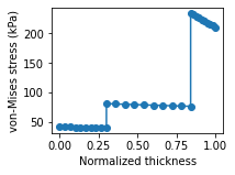
Lastly, we can calculate the Cauchy stress tensor through the thickness of the artery at a given internal radius (which is equal to the value we calculated at a pressure of 15). It returns a tuple of normalized thickness xi and a list of stresses stress.
[12]:
xi,stress = artery.cauchy_stress(6.97341844)
To visualize the results, we calculate the von-Mises stress for each tensor in the list stress and then plot it. We note the jump in stress at the interface, which is because of the incompatible reference states of the three layers. Note that here the reference state of each layer is the same (same radius and opening angle), however they are still incompatible, since for compatibility, the outer radius of innermost layer should be equal to the inner radius of the next layer, and so on.
[13]:
def von_mises(sigma_list):
    return [np.sqrt(3./2.)*np.linalg.norm(sigma-np.trace(sigma)/3.*np.eye(3)) for sigma in sigma_list]

fig,ax = plt.subplots(1,1,figsize=(4*0.7,3*0.7))

ax.plot(xi,von_mises(stress),'-o')
ax.set_xlabel('Normalized thickness')
ax.set_ylabel('von-Mises stress (kPa)')
plt.show()