Tutorial: simple uniaxial test
Material creation
We start by importing the library and creating a neo-Hookean material model
[1]:
import pymecht as pmt
mat = pmt.MatModel('nh')
We can access the parameters of the material model and print them. It shows that the parameters are of type ParamDict which includes their current value, whether they are fixed or not, and their lower/upper bounds (if applicable).
[2]:
mat_params = mat.parameters
print(mat,mat_params)
Material model with 1 component:
Component1: NH
 ------------------------------------------------------------------
Keys              Value       Fixed?      Lower bound Upper bound
------------------------------------------------------------------
mu_0              1.00        No          1.00e-04    1.00e+02
------------------------------------------------------------------
Sample creation
Next we can create a uniaxial extension sample from the material and print its parameters, which will include the material parameters as well as the geometric parameters (length and cross-sectional area)
[3]:
sample = pmt.UniaxialExtension(mat)
sample_params = sample.parameters
print(sample)
print(sample_params)
An object of type UniaxialExtensionwith stretch as input, force as output, and the following material
Material model with 1 component:
Component1: NH

------------------------------------------------------------------
Keys              Value       Fixed?      Lower bound Upper bound
------------------------------------------------------------------
L0                1.00        No          1.00e-04    1.00e+03
A0                1.00        No          1.00e-04    1.00e+03
mu_0              1.00        No          1.00e-04    1.00e+02
------------------------------------------------------------------
Simulation by setting parameters
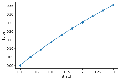
We can set the parameters values to what we would like and then apply a stretch to the sample to calculate the force. We import numpy and matplotlib libraries for the stretch vector and plotting the force-strech plot.
[4]:
import numpy as np
from matplotlib import pyplot as plt

sample_params.set('mu_0',5)
sample_params.set('A0',0.1)
sample_params.set('L0',10)
applied_stretch = np.linspace(1,1.3,10)
force = sample.disp_controlled(applied_stretch,sample_params)
plt.plot(applied_stretch,force,'-o')
plt.xlabel('Stretch')
plt.ylabel('Force')
plt.show()
Parameter fitting
If we have some force measurements (say from experiments), we can also do parameter fitting. We should fix the values of A0 and L0 to ensure a unique solution.
[5]:
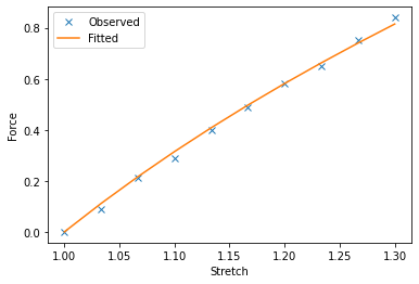
force_measured = np.array([0,0.09,0.21,0.29,0.4,0.49,0.58,0.65,0.75,0.84])
def sim_func(params):
    force_modeled = sample.disp_controlled(applied_stretch,params)
    return force_modeled

sample_params.fix('A0')
sample_params.fix('L0')
param_fitter = pmt.ParamFitter(sim_func,force_measured, sample_params)
param_fitter.fit()
print("Results after fitting")
print(sample_params)
plt.plot(applied_stretch,force_measured,'x',label='Observed')
plt.plot(applied_stretch,sim_func(sample_params),'-',label='Fitted')
plt.xlabel('Stretch')
plt.ylabel('Force')
plt.legend()
plt.show()
Parameter fitting instance created with the following settings
------------------------------------------------------------------
Keys              Value       Fixed?      Lower bound Upper bound
------------------------------------------------------------------
L0                10.00       Yes         -           -
A0                0.10        Yes         -           -
mu_0              5.00        No          1.00e-04    1.00e+02
------------------------------------------------------------------

1 parameters will be fitted.
   Iteration     Total nfev        Cost      Cost reduction    Step norm     Optimality
       0              1         4.1049e-01                                    1.20e+01
       1              2         2.2983e-02      3.88e-01       5.00e+00       2.62e+00
       2              3         1.0599e-03      2.19e-02       1.48e+00       4.24e-02
       3              4         1.0540e-03      5.94e-06       2.48e-02       1.19e-05
       4              5         1.0540e-03      4.65e-13       6.93e-06       2.01e-10
`gtol` termination condition is satisfied.
Function evaluations 5, initial cost 4.1049e-01, final cost 1.0540e-03, first-order optimality 2.01e-10.
Fitting completed, with the following results
------------------------------------------------------------------
Keys              Value       Fixed?      Lower bound Upper bound
------------------------------------------------------------------
L0                10.00       Yes         -           -
A0                0.10        Yes         -           -
mu_0              11.51       No          1.00e-04    1.00e+02
------------------------------------------------------------------

Results after fitting
------------------------------------------------------------------
Keys              Value       Fixed?      Lower bound Upper bound
------------------------------------------------------------------
L0                10.00       Yes         -           -
A0                0.10        Yes         -           -
mu_0              11.51       No          1.00e-04    1.00e+02
------------------------------------------------------------------
Random Parameters: Monte Carlo simulation
We can also approach the problem probabilistically by treating the parameteres as random variables. Either we can generate samples RandomParameters and propagate them through the model (Monte Carlo simulation).
[6]:
random_params = pmt.RandomParameters(sample_params)
print(random_params)
random_samples = random_params.sample(300)
print('random_samples are a list of parameters dictionaries:', type(random_samples),len(random_samples))
results = np.array([sim_func(s) for s in random_samples])
print('results are of shape', results.shape)
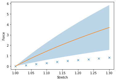
#We can plot the mean and variation of these
mean = np.mean(results,axis=0)
sd = np.std(results,axis=0)
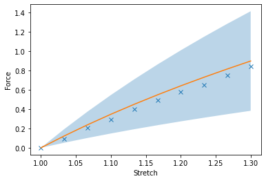
plt.plot(applied_stretch,force_measured,'x',label='Observed')
plt.plot(applied_stretch,mean,'-')
plt.fill_between(applied_stretch,mean-sd,mean+sd,alpha=0.3)
plt.xlabel('Stretch')
plt.ylabel('Force')
plt.show()
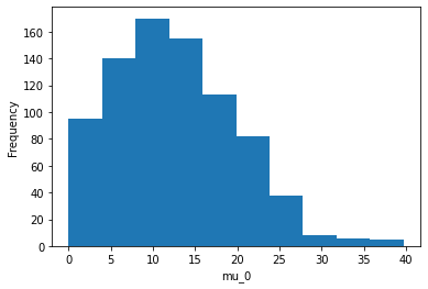
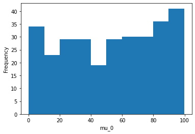
mu_samples = [s['mu_0'] for s in random_samples]
plt.hist(mu_samples,bins=10)
plt.xlabel('mu_0')
plt.ylabel('Frequency')
plt.show()
Keys              Type              Lower/mean        Upper/std
------------------------------------------------------------------------
L0                fixed             10.00             10.00
A0                fixed             0.10              0.10
mu_0              uniform           1.00e-04          1.00e+02
------------------------------------------------------------------------

random_samples are a list of parameters dictionaries: <class 'list'> 300
results are of shape (300, 10)
Random parameters: Markov Chain Monte Carlo simulation
Or we can perform a Markov Chain Monte Carlo (MCMC) simulation through some likelihood function.
[7]:
def prob(params):
    force_modeled = sample.disp_controlled(applied_stretch,params)
    diff = force_modeled - force_measured
    diff_norm2 = np.dot(diff,diff)
    var = 2.
    prob = np.exp(-diff_norm2/2./var) #in the case of MCMC we can skip the proportionality factor
    return prob,force_modeled

mcmc = pmt.MCMC(prob,sample_params)
MCMC instance created with the following settings
------------------------------------------------------------------
Keys              Value       Fixed?      Lower bound Upper bound
------------------------------------------------------------------
L0                10.00       Yes         -           -
A0                0.10        Yes         -           -
mu_0              11.51       No          1.00e-04    1.00e+02
------------------------------------------------------------------

1 parameters will be varied.
[8]:
mcmc.run(1000)
100%|████████████████████████████████████████████████████████████████████████████████████████████| 1000/1000 [00:00<00:00, 2575.02it/s]
MCMC sampling completed. Acceptance rate: 0.812
Number of samples: 812
To access the samples, use get_samples()
[9]:
mcmc_samples = np.array(mcmc.get_samples()) #convert the list into an array
mcmc_probs = np.array(mcmc.get_probs()) #convert the list into an array
mcmc_force = np.array(mcmc.get_values()) #convert the list into an array
print(np.array(mcmc_force).shape)
#We can plot the mean and variation of these
mean = np.mean(mcmc_force,axis=0)
sd = np.std(mcmc_force,axis=0)
plt.plot(applied_stretch,force_measured,'x')
plt.plot(applied_stretch,mean,'-')
plt.fill_between(applied_stretch,mean-sd,mean+sd,alpha=0.3)
plt.xlabel('Stretch')
plt.ylabel('Force')
plt.show()

plt.hist(mcmc_samples)
plt.xlabel('mu_0')
plt.ylabel('Frequency')
plt.show()
(812, 10)